Build a Speaker Recognition Model Using MLOps Tools

This is the first post of this series, so I will try to illustrate the overall landscape of the acoustic domain via one of the classical problems. This blog go through data variety, input type and model building.

Data Variety

Voice includes lots of variety even though people speak the same transcript. You can distinguish two voices who speak from two different people. Even for the same person, voices can be different when you have different emotions (e.g., happy, angry, sad, etc.).

Input Type

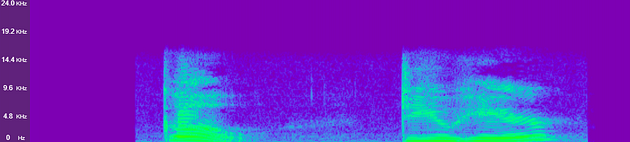
We may feed bytes, characters, or tokens into a text-based ML model. On the other hand, we can feed waveform or spectrogram into an acoustic ML model. A spectrogram is a visualization of representing the signal (i.e., voice) strength (i.e., loudness) of a signal over time at various frequencies.

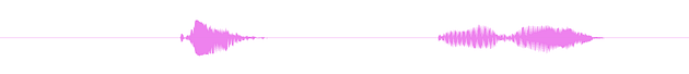
In exploratory data analysis, it is not that hard to explore characters or tokens. Unlike text, we can not visualize audio clips directly. Waveform and spectrogram visualization is a good way to understand our data.

You may use audio-preview plugin (if you are using Visual Studio), native software on your machine, or Jupyter Notebook (with librosa) to understand it. Alternatively, we may use cloud solutions to achieve the same purpose. For example, once uploading files to DagsHub, everyone with access is able to listen and visualize it via browser.

Lots of modern ML models consume spectrograms (or mel-spectrograms) instead of waveforms for several reasons. Waveform includes more information but spectrogram are closed to the human auditory system. Another reason is that we can reuse computer vision model architecture on the acoustic models. I will show how to use the computer vision (CV) architecture, ResNet [1], and speaker recognition model later.

Speaker Recognition

Our toy problem is speaker recognition. Given voice input, we want to identify the speaker. It is similar to facial recognition and finger recognition when you try to unlock your iPhone.

Both speaker verification and identification are under the speaker recognition umbrella. Speaker identification refers to determining who the enrolled speaker is. Speaker verification means either accepting or rejecting the identity claimed by a speaker.

Dataset

In the regression problem, we have the titanic dataset. In audio problems, I usually start from the LibriSpeech dataset [2]. You may download it from OpenSLR, PyTorch, TensorFlow, or HuggingFace.

Although we can download it from the internet easily, it is raw audio data (i.e., waveform). As mentioned in the previous section, we feed spectrogram data to ML models instead of waveform data. You may convert waveform data to spectrogram and persist in your local machine. It is fine if you work alone without any scale requirement. Another option is uploading it to a cloud provider (e.g., AWS, GCP), but you have to manage it by yourself.

Alternatively, you may consider using the Direct Data Access feature which is provided by DagsHub. It helps us to streamline the process of uploading and downloading from the cloud. We can focus on model training rather than infrastructure.

The following codes show how to upload files to DagsHub’s cloud.

# Initialize remote date repository
from dagshub.upload import Repo
repo = Repo(repo_owner, repo_name)
dataset_dir = 'datastore'
ds = repo.directory(dataset_dir)

# Iterlate local audio file paths
for f in audio_file_paths:
    file_name = os.path.basename(f)
    _id, session, _ = file_name.split('-')
    
    remote_file_path = os.path.join(
        'LibriSpeech',
        _id,
        session,
        file_name
    )
    
    # Upload file
    ds.add(file=f, path=remote_file_path)

# Commit change on files upload
ds.commit(f"Upload {total_cnt} audio files", versioning="dvc")

After talking about data storage, we will move to data processing. Converting waveform to mel-spectrogram is a very typical process, and most of the models consume it. Therefore, you may consider caching the processed result.

Data Processing

librosa [3] is a famous python package for music and audio analysis. It provides an easy way to convert raw waveform data to mel-spectrogram data.

from dagshub.streaming import DagsHubFilesystem
fs = DagsHubFilesystem()

import csv

metadata = {}
with fs.open('datastore/LibriSpeech/metadata.csv') as infile:
    reader = list(csv.reader(infile))
    for row in reader[1:]:
        metadata[row[0]] = len(metadata)

Sample rate means the number of samples per second. For example, 16000 means there are 16000 data points per second. Higher sample rates include more data points. 16000, 22050, 44100, and 48000 are sample rates that I usually use.

When working on audio data, it will be good to have the same sample rate across all data feeding into the ML model. Passing sample_rate into librosa.load function, which helps to convert the audio clip to the expected sample rate.

Modeling

I mentioned we could leverage CV model architecture on the acoustic model. Simply load the ResNet34 model by using torchvision package, we have the pre-trained model now.

# Load audio data
y, sr = librosa.load(file_path, sr=sample_rate)
# Convert waveform to mel-spectogram
spec=librosa.feature.melspectrogram(y=f.numpy(), sr=sample_rate)
# Convert a power spectrogram (amplitude squared) to decibel (dB) units
spec_db=librosa.power_to_db(spec)

Tracking

Experiment tracking is very important when building a model. It allows us to compare model metrics (performance, training time, etc) against different settings. You can mark it down into a spreadsheet or use experiment tracking tools. Weights & Biases, Comet ML, MLflow are some of the great tools that we can use.

We do not need extra tools if we use DagsHub as you just need to run a few lines of code (auto-tracking is available for some frameworks such as PyTorch Lighting) to create the experiment tracking.

from torchvision.models import resnet34
import torch.nn as nn
# Load ResNet34 CV model
resnet_model = resnet34(weights=True)
# Adjusted the last layer output for our binary classification use case
resnet_model.fc = nn.Linear(512, label_cnt)
# Adjust the first convolution neural network (CNN) layer for our use case
resnet_model.conv1 = nn.Conv2d(
  1, 
  64,
  kernel_size=(7, 7),
  stride=(2, 2), 
  padding=(3, 3), 
  bias=False
)

Model Registry

Besides metrics, we also want to keep the trained model, as we may need to load it later. Model Registry is another important section that we need to take care of. We can simply save the model locally or upload it to the cloud (e.g., AWS, Azure, GCP). However, management is needed but not just storing the file. For example, the association between the experiment and the model is needed. Model access control is suggested as we may only want to share our model with the targeted group of people but not all.

Same to the dataset, we can upload the model to DagsHub so that we have a single view to access the code, experiment, and model.

from dagshub import DAGsHubLogger
logger = DAGsHubLogger(
  metrics_path="logs/test_metrics.csv", 
  hparams_path="logs/test_params.yml"
) 
logger.log_hyperparams({
    'learning_rate':learning_rate,
    'optimizer': 'adam',
    'epoch': 3,
    'loss': 'ce'
})

accuracy = evaluate(model, x, y_true)
logger.log_metrics({'accuracy': accuracy})

Take Away

Having a centralized place to keep tracking code, experiment, and model helps us to focus on the model rather than MLOps. A model builder is an expert in training a good model for the company but may not be good at building MLOps infrastructure.

Here is the full script for the model training. To balance the optimization and readability, we simplify the flow such as data streaming, data processing, and modeling. There are a few things that we can further optimize the data processing part. Instead of streamlining data at the very beginning, we should load data on demand to maximize the Direct Data Access feature. Also, we may introduce data augmentation if a more generalized model is needed. To maximize DagsHub Storage feature, we can preprocess (i.e. convert waveform to spectrogram) data and upload it instead of processing data every time.

Here is the repo for the datastore, experiment tracking, and model registry. You may access it to understand how we can combine everything together.

Like to learn?

I am Data Scientist in Bay Area. Focusing on the state-of-the-art in Data Science, Artificial Intelligence, especially in NLP and platform related. Feel free to connect with me on LinkedIn or Github.

Reference

[1] He et al. (2015). Deep Residual Learning for Image Recognition
[2] Panayotov et al. (2015). LibriSpeech: An ASR corpus based on public domain audio books
[3] McFee et al. (2015). librosa: Audio and Music Signal Analysis in Python