Active Learning Your Way to Better Models

The world is currently experiencing a machine learning boom, which is in large part thanks to the effectiveness of deep learning models. The success of deep learning can be traced to the internet.

The internet is the reason we have so much data, with which to train these models. Without the internet, there is no access to the digital information we need to learn and extract patterns from. The internet is Big Data.

If Ben Parker had been a data scientist, he might have told Peter:

With big data, comes big problems

The internet makes it almost too easy to collect data. Just collecting data, however, is useless. We need a way to label it.

Labeling so much data can be difficult and expensive. In fact, labeling all of the data is often pointless. Not all data are created equal. Good, high quality data can improve a model significantly, while low quality data may even hinder a models ability to learn.

So how do we sift through the steaming pile of data to find the good samples we need for our model?

One effective answer is active learning.

What is Active Learning?

Active learning is semi-supervised learning with a human-in-the-loop. The main difference to standard supervised learning is that rather than having humans label all training data, an algorithm or model chooses which data should be labeled.

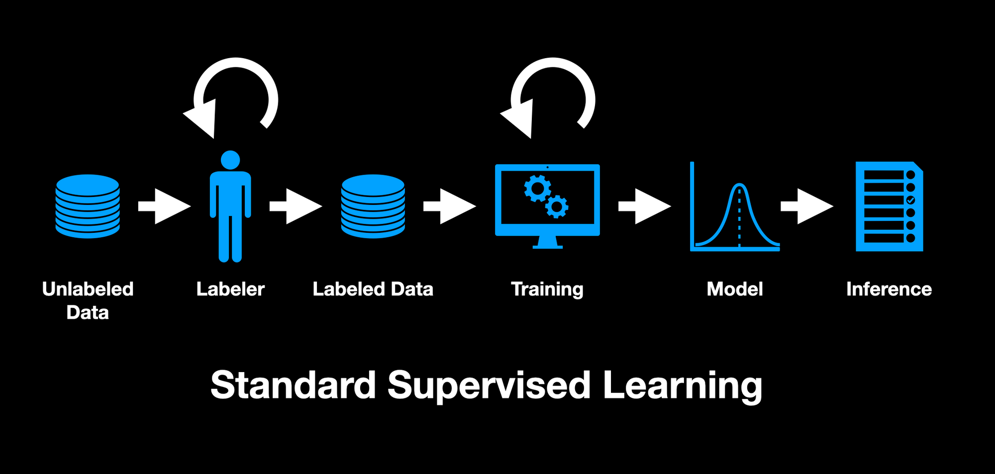
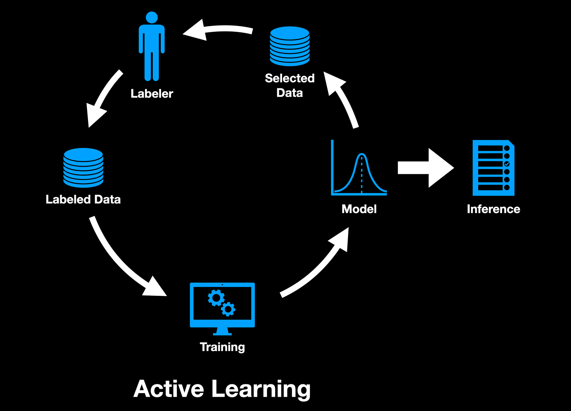
This makes active learning a data-centric approach to machine learning, where we hold the code static and iterate on the data. The active learning model's goal is to maximize information gained from as few data points as possible. In doing so, it generally picks the more difficult and troublesome data to learn from.

We can kind of think of it like a student studying for an exam. If the student chooses to only practice the easiest example problems, which may be covered in the exam, they miss out on understanding crucial concepts. However, if the student specifically focuses on example problems, which are difficult for them, they will more likely learn more and do better overall on the exam.

The natural question that comes to mind, though, is how does the algorithm choose which data it should focus on?

Data Sampling

When getting started with active learning, the question of how to sample the data can be daunting or confusing. However, there is no shortage of options to choose from. Thankfully, each one also tends to be intuitively understandable.

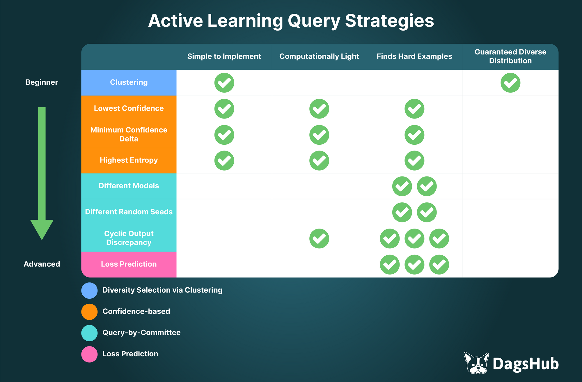
Diversity Selection via Clustering

If we can use an unsupervised algorithm to cluster the data, like k-means clustering, we can then sample training data from each cluster. While this doesn't necessarily choose difficult training data, it does help to ensure that our dataset is diverse. It will be less likely to miss important categories of data.

This method is also a possible way to get the initial dataset to train our model, since the rest of the data sampling techniques require us to already have a model to determine which data should be sampled.

This sounds like the basis for a sequel to Inception 🤔

Confidence-Based

Possibly the easiest data sampling technique to implement are confidence based ones. And since we're often creating machine learning models to automate something to make our jobs easier, this is a popular route to take.

Three main confidence-based sampling techniques are:

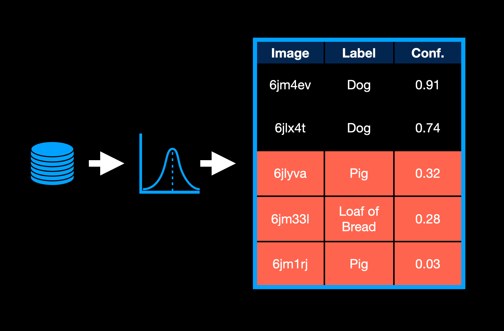
1. Lowest Confidence

For this technique, we’d like to find the samples, where the model is least confident about its answer. This corresponds to the examples the model is struggling to classify. It is having trouble even recognizing the underlying data.

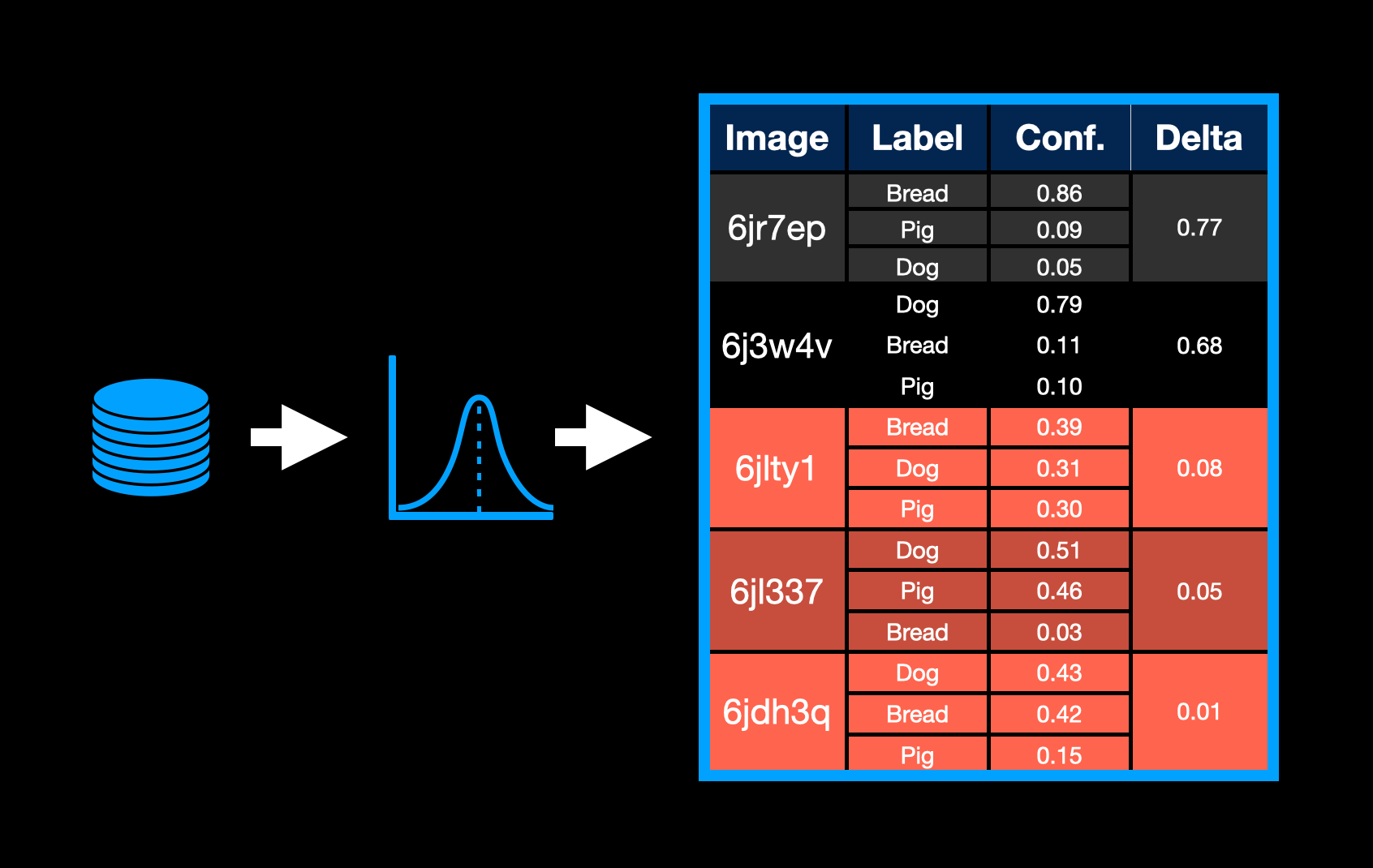
2. Minimizing Confidence Delta

Another technique is to find samples, where the top two labels have very similar confidences. We do this by calculating the delta between them and choosing those samples with the smallest differences, as shown by the highlighted rows in the table below.

This is an indication that the model is having a hard time deciding, which category a sample belongs to. These samples are, therefore, very likely complex examples.

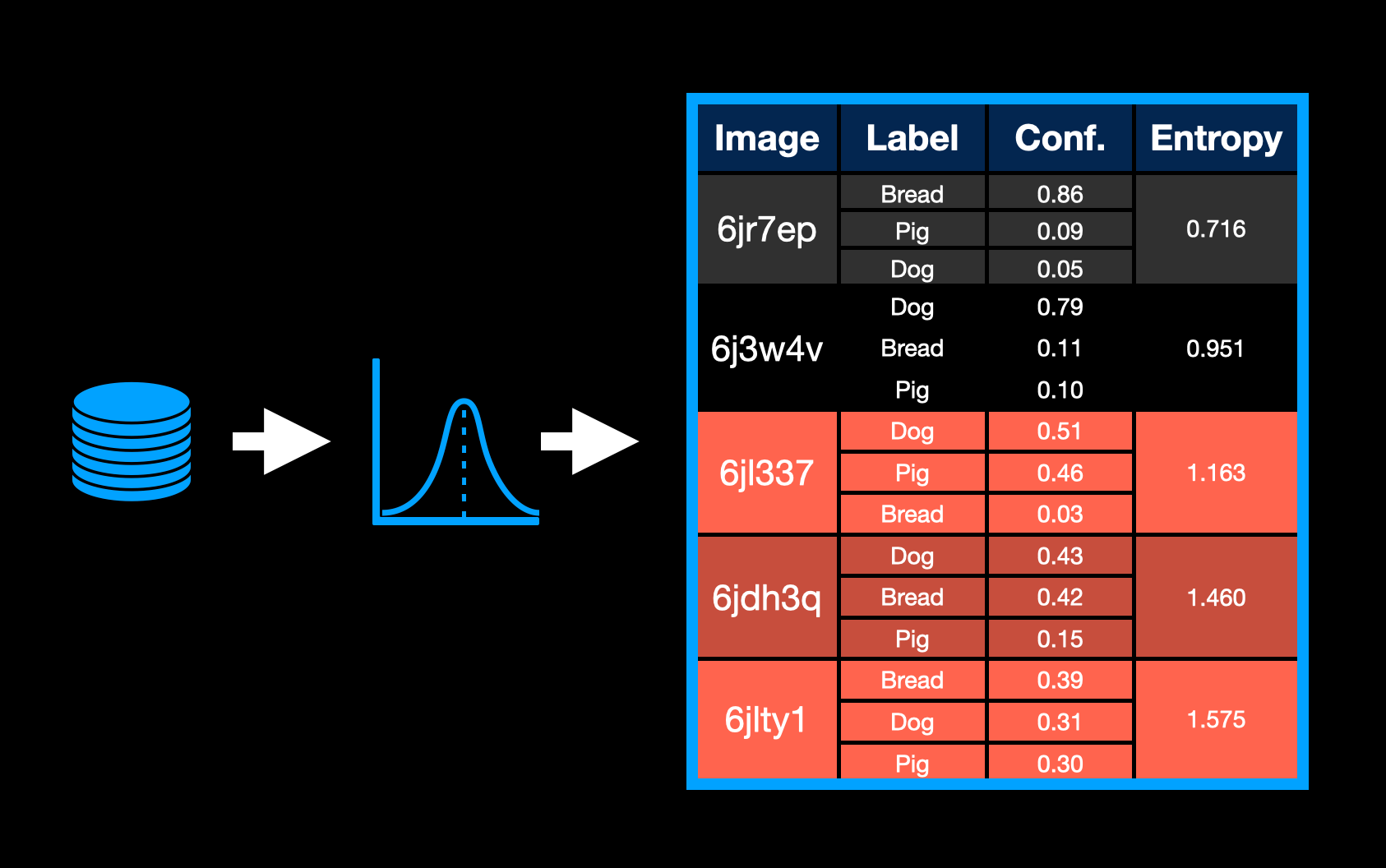
3. Entropy

Entropy is a measure of the confidence across all categories. The larger the entropy, the less sure a model is overall about the data. This is often written as the following equation:

\[H(X)=-\sum_{i=1}^n p(x_i)\log p(x_i)\]

A version of this formula comes up in many fields, including physics, statistics, and engineering. It may also look familiar, if you remember the details of how cross-entropy loss functions work.

Here:

• \(\boldsymbol{n}\) is the number of label categories
• \(\boldsymbol{x_i}\) is the \(\boldsymbol{i^{th}}\) label category
• \(\boldsymbol{p(x_i)}\) is the probability that the data belongs to the \(\boldsymbol{x_i}\) category

By maximizing entropy, we select the most confusing data for the model that should be labeled.

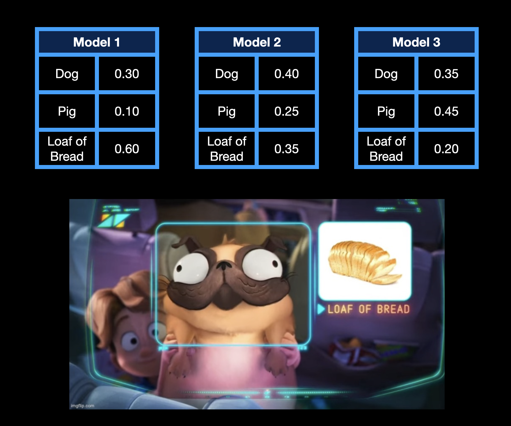
Disagreement Among Multiple Models

Another fantastic method to sample our data is to use the power of democracy. We can simply have multiple models and let them vote on which data should be labeled! This is also known as Query-by-Committee.

There are a couple of different ways, in which we could do this:

1. Different Models - Train two or more different models on the same initial dataset and find new data, for which they disagree the most. These different models can also vary wildly — different neural network architectures, decision trees, support vector machines. The important thing is that each model learns something slightly different about the target labels. Voting is pointless if there are no differences of opinions!
2. Different Random Seeds - Train multiple copies of the same model, but use different random seeds for each one.
3. Cyclic Output Discrepancy - Use consecutive iterations of the same model to determine which data is disagreed upon most. Each iteration is an entire active learning cycle. For this method, we iterate on a single model.

Loss Prediction

Another query selection option is to try to predict what the loss will be for a given sample. To do this, we could create a double branch network.

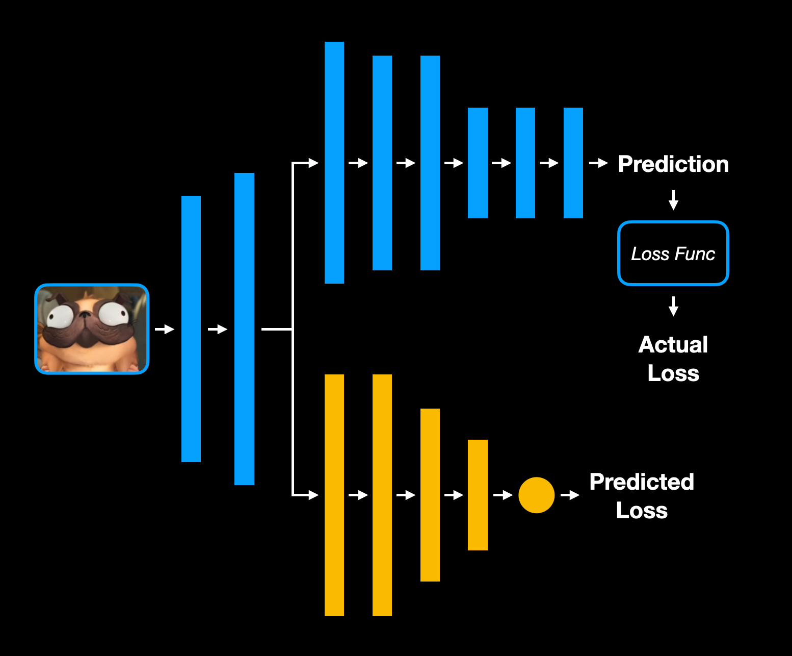
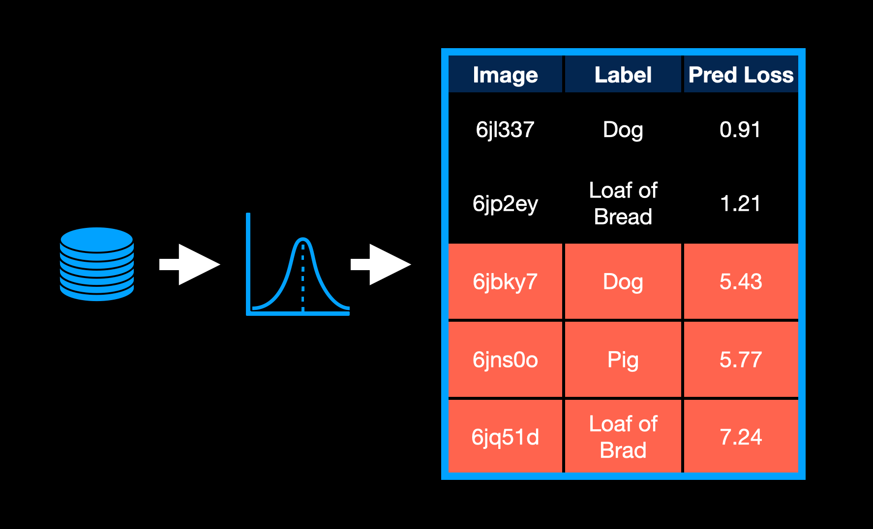
The main branch is our desired model and the second branch is a regression model, which predicts the loss based on the input. Using the loss-prediction branch, we can then choose samples with the largest loss value to label.

Training a Loss Prediction Network

You might be thinking to yourself, how do I train this double branch network, if it's improving loss while trying to predict it? That is an excellent question!

The authors of Loss-based active learning via double-branch deep network discuss their training methodology. They used two copies of the main branch of the network. One, called the Target Model and the other the Training Model. The Target Model is held constant for each epoch and is used to determine the ground truth loss value for the input samples. The Training Model is continuously trained for the original objective (classification, object detection, segmentation, etc.).

At the end of every epoch, the weights from the Training Model are copied exactly to the Target Model. This way, the ground truth loss values are consistent across the epoch, but the model can still be trained.

Benefits of Active Learning

Active learning is not a hammer we want to use on all problems.

However, there are many reasons to use it and situations where it can be extremely beneficial.

The main benefit of active learning is that it allows us to label less data. Our data goes a lot further than in standard supervised machine learning.

Imagine the situation where we are training a model to help domain experts be more efficient. Experts can be doctors looking at x-rays, agronomists determining the health of crops, astrophysicists trying to find exoplanets, etc...

There is a catch-22 here, though. We need these domain experts to label the data, but these experts' time is too precious (and expensive) to be spent labeling data.

Training non-experts to label the data is an option, but this is time-consuming, expensive, and more prone to error. Instead, by using active learning, we can minimize the amount of time domain experts spend labeling data.

Additionally, active learning can lead to higher accuracy models. Here is where the phrase garbage in, garbage out makes a lot of sense.

If a lot of our data is not helpful, or worse, incorrectly labeled, this can decrease the overall accuracy of the model. A recent MIT study found an error rate of about 5.8% on ImageNet’s validation dataset! Additionally, a group, who wrote a tool to detect duplicates, anomalies, and incorrect labels in datasets, have discovered that ImageNet-21k includes 1.2 million duplicates! That is about 8.5% of the dataset 😱

These errors make models trained on them measurably worse. Active learning also allows us to cover more edge cases efficiently, which improves accuracy.

Finally, less data, which is higher quality, leads to a knock-on effect. When we have less data to train, we save on compute time. And by using active learning, our data is high quality, which helps models converge faster. This makes models cheaper and quicker to retrain later on.

Drawbacks of Active Learning

There's no such thing as a free lunch. Active learning does have drawbacks, which need to be overcome.

Active learning adds complexity to our machine learning workflow. The setup and engineering of the project are more complicated, since there are few turn-key solutions out there. This means, more room for bugs and errors in code. This complexity also means active learning can be slower to get initial results.

When using active learning, there is also the potential for the model to focus on outliers. Outliers are likely to be chosen by any of the query strategies, so our experts need to be cognizant of that and just mark any outlier data as such. Including a data validation step after the model selects examples to label, will help us prevent outliers from creeping into our labeled dataset.

Additionally, since active learning is sampling data from an entire collected dataset, the distribution of the sampled data will not necessarily match the distribution of the entire dataset. In many ways, this is desirable. However, we need to understand that there is a risk of sampling bias being introduced. This can be difficult to detect and debug.

Conclusion

Phew! If you're new to active learning, this was probably a lot of information to take in.

While reading this article you learned:

• what active learning is
• various data sampling (querying) strategies used with active learning
• benefits of, and...
• ...disadvantages to active learning

As this article is theoretical in nature, we recommend finding a pet project you can put this new knowledge into practice. By implementing active learning yourself, you'll solidify your understanding of the concepts from this article.

In a future post we will walk through such a project, in case you need more inspiration 😉

Thanks for reading! If you have any questions, feel free to reach out.

References:

1. W. H. Beluch, T. Genewein, A. Nürnberger, J. M. Köhler. The power of ensembles for active learning in image classification. CVPR 2018.
2. Siyu Huang, Tianyang Wang, Haoyi Xiong, Jun Huan, Dejing Dou. Semi-Supervised Active Learning with Temporal Output Discrepancy. ICCV 2021. arXiv:2107.14153 [cs.CV]
3. Donggeun Yoo, In So Kweon. Learning Loss for Active Learning. CVPR 20219. arXiv:1905.03677 [cs.CV]
4. Qiang Fang, Dengqing Tang. Loss-based active learning via double-branch deep network. International Journal of Advanced Robotic Systems. 18 (5).
5. Curtis G. Northcutt, Anish Athalye, Jonas Mueller. Pervasive Label Errors in Test Sets Destabilize Machine Learning Benchmarks. arXiv:2103.14749 [stat.ML]