Using data validation techniques to investigate the impact of data resampling

When dealing with imbalanced data, one of the go-to approaches is to resample the training data to reduce the class imbalance. This can involve undersampling the majority class, oversampling the minority class, or a combination of both. To make it even more interesting, there are many approaches we can follow for each of the three mentioned categories of methods.

One of the well-known disadvantages of resampling the training data is that we distort the initial distribution of features and the relationships between them. Naturally, we might be perfectly fine with that as long as the performance of our models improves. However, it would be interesting to know how severe the problem actually is. There are many ways to check that, for example, with simple visualizations (which are not feasible with a very high-dimensional dataset), or by inspecting the correlation matrix.

In this article, we will take a bit of an off-the-beaten-track approach and use the deepchecks library to compare the original dataset with the resampled one. We will investigate the difference between three resampled datasets using the popular credit card fraud dataset. Let’s dive right into it!

Data

We will be using one of the most popular imbalanced classification datasets available, that is, the credit card fraud dataset (available at Kaggle). We summarize the relevant information in the following points:

• the dataset contains credit card transactions carried out over a period of two days in September 2013 by European cardholders.
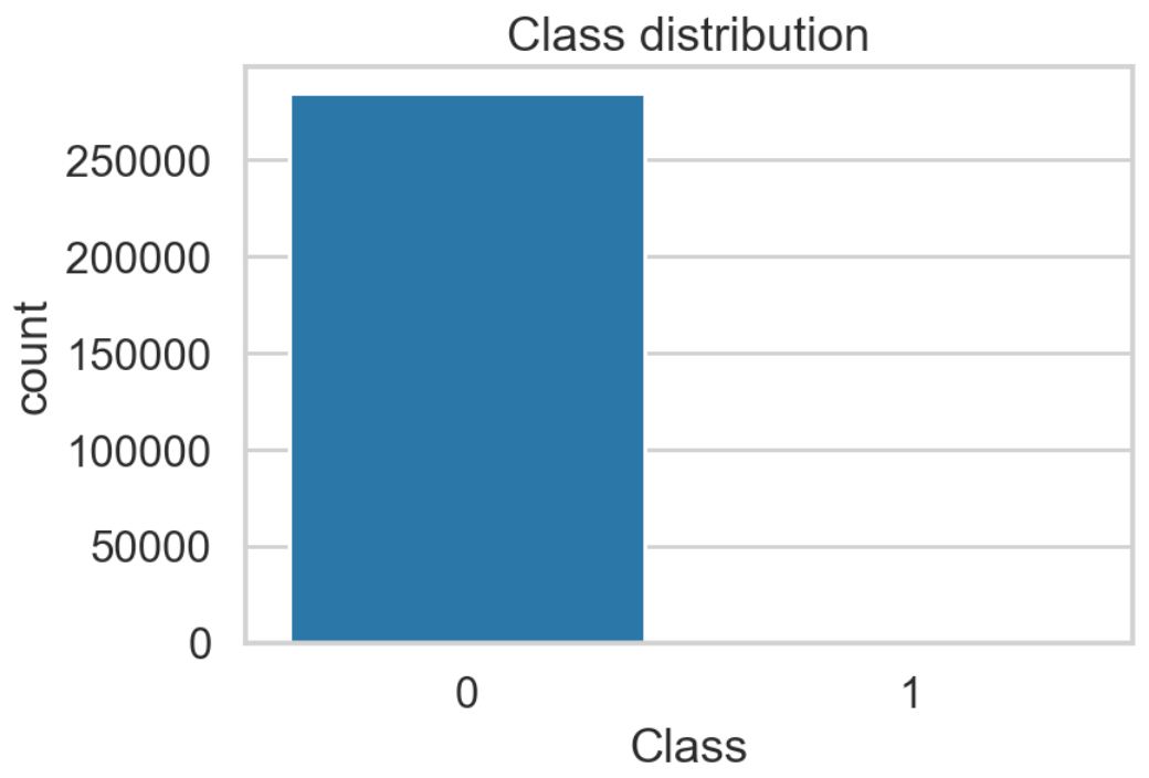
• the dataset is highly imbalanced — out of  284,807 transactions, 492 were identified as fraudulent. That corresponds to 0.173% of all transactions.
• in order to anonymize the data, the dataset contains 28 numerical features which are the result of a PCA transformation. The only features that were not anonymized are Time (seconds elapsed between each transaction and the first transaction in the dataset.) and Amount (the transaction’s amount). This results in a total of 30 features.

Considered resampling techniques

In this article, we explore three popular  resampling techniques. There are many great articles out there describing the nitty-gritty details of algorithms such as SMOTE, hence we only focus on providing a brief refresher.

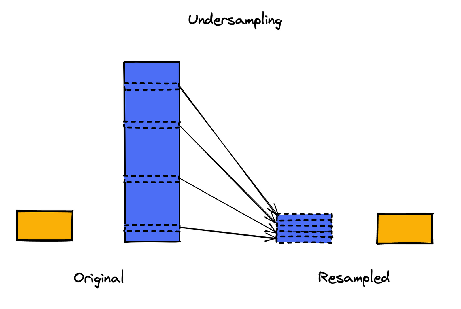
1. Random undersampling

Random undersampling is the simplest of the available undersampling approaches. We draw random samples (by default without replacement) from the majority class until we obtain a 1:1 ratio of the classes. The biggest issue with this approach is the information loss caused by discarding the majority of the training set.

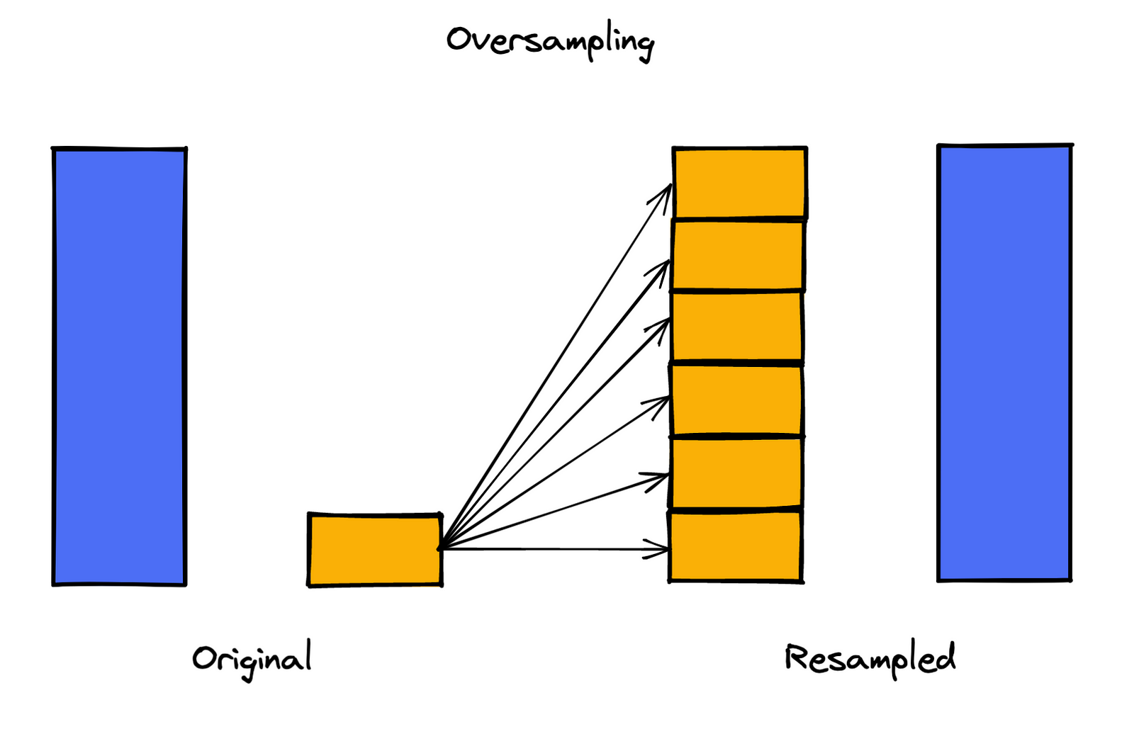
2. Random oversampling

The oversampling equivalent of random undersampling. Here, we draw samples with replacement from the minority class until the desired ratio of the classes is achieved. While it does not cause information loss, it comes with the danger of overfitting, which is  caused by replicating observations from the minority class.

3. SMOTE

SMOTE (Synthetic Minority Oversampling Technique) is an oversampling technique that creates new, synthetic observations from the minority class. This way, the algorithm avoids the problem of overfitting encountered with random oversampling.

The algorithm executes the following steps:

• choose an observation from the minority class.
• identify its k-nearest neighbors.
• create synthetic observations on the lines connecting (interpolating) the selected observation to the nearest neighbors.
• repeat the steps above until the desired ratio of the classes is reached.

While it does not cause information loss and tries to account for the overfitting, SMOTE is unfortunately not a silver bullet to imbalanced classes. The algorithm comes with its own set of drawbacks. The biggest one is that it can introduce more noise to the data and cause overlapping of minority and majority classes (the infamous bridges between the observations). The reason for that is that SMOTE does not take into account the observations from the majority class while creating the new observations.

Deepchecks

deepchecks is an open-source Python library that allows for testing and validating both data and the performance of ML models. It does so by, among others, verifying the data  integrity, inspecting distributions, validating its splits, etc.

While working with deepchecks, we can use the handy concept of suites (sets of checks), which make working with the library quite effortless. For tabular data, we can use the following suites:

• single_dataset_integrity — this suite is aimed at exploring a single dataset (before any splits). It focuses on verifying the data’s integrity by, for example, checking the number of duplicated observations, if there are any issues with the categorical features, detecting outliers, etc.
• train_test_validation — this suite is intended for investigating whether any data split (the most common example is the train-test split) results in representative datasets. Examples include: investigating the class distribution/balance, checking if there is no significant change in distributions between the features or labels in each of the classes, looking out for potential data leakage, etc.
• model_evaluation— this suite is intended for evaluating the performance of an ML/DL model. Using it we can examine several performance metrics, compare the performance to benchmarks, etc.

We can also use the full_suite, which combines the three suites mentioned above. For our convenience, the library automatically selects which tests from the three suites are relevant for our use case.

For our example, we are mostly interested in the functionalities of the train_test_validation suite, but we will use the full_suite to also examine some data integrity checks.

Preparing the data comparisons

In this section, we describe how to process the data and resample it using the considered techniques. We start by specifying the directories for storing the data at various steps and the intended location for the data validation reports.

# directories
RAW_DIR = "data/raw"
PROCESSED_DIR = "data/processed"
AUGMENTED_DIR = "data/augmented"
REPORTS_DIR = "data_validation"

Our data is located in three directories:

• raw — here we store the original data downloaded from Kaggle.
• processed — here we store the data after the train-test split.
• augmented — here we store the resampled datasets. It is important to keep in mind that when resampling, we only resample the training data!.

Additionally, we track the data using DVC. You can read more about setting up data versioning with DVC in my other article.

In the following script, we load the data from the raw directory, separate the features from the target, drop the Time feature, split the data into training and test sets (using the 80–20 ratio), and then save it to the processed directory. When working with imbalanced classes, it is crucial to apply the stratified train-test split, so the proportions of classes in the datasets are preserved.

After the split, we have also applied scaled the Amount feature using scikit-learn’s RobustScaler. As we have mentioned before, all the other 28 features are obtained from running the PCA, so we assume that their values were scaled appropriately before the transformation.

In this project, we will be using a Random Forest classifier, which does not require explicit feature scaling. However, resampling algorithms such as SMOTE use k-Nearest Neighbors (kNN) under the hood. For those distance-based algorithms the scale does matter.

import pandas as pd 
from config import RAW_DIR, PROCESSED_DIR
import os

from sklearn.preprocessing import RobustScaler
from sklearn.model_selection import train_test_split 

# load data
df = pd.read_csv(f"{RAW_DIR}/creditcard.csv")

# separate the target
X = df.copy() 
y = X.pop("Class")

# dropping unnecessary feature
X = X.drop(columns=["Time"])

# stratified train-test split
X_train, X_test, y_train, y_test = train_test_split(X, y,  
                                                    random_state=42,
                                                    test_size=0.2,  
                                                    stratify=y) 

# sanity check 
print(y_train.value_counts(normalize=True).values)
print(y_test.value_counts(normalize=True).values)

# scale the amount feature
robust_scaler = RobustScaler()
X_train[["Amount"]] = robust_scaler.fit_transform(X_train[["Amount"]])
X_test[["Amount"]] = robust_scaler.transform(X_test[["Amount"]])

# prepare output dir
os.makedirs(PROCESSED_DIR, exist_ok=True)

# saving data
X_train.to_csv(f"{PROCESSED_DIR}/X_train.csv", index=None)
X_test.to_csv(f"{PROCESSED_DIR}/X_test.csv", index=None)
y_train.to_csv(f"{PROCESSED_DIR}/y_train.csv", index=None)
y_test.to_csv(f"{PROCESSED_DIR}/y_test.csv", index=None)

In the next step, we apply various resampling techniques (available in the imbalanced-learn library) to the training data and store the results in the augmented directory. To make the code easy to extend, we defined the list of resampling techniques, and the script iterates over it. This way, we can easily experiment with other approaches to resampling, for example, ADASYN. Alternatively, we can use different parameters for the algorithms. In the case of SMOTE, we could specify the number of nearest neighbors to consider while creating the synthetic data points.

import os 
import pandas as pd 
from config import RAW_DIR, PROCESSED_DIR, AUGMENTED_DIR

from imblearn.over_sampling import RandomOverSampler, SMOTE, ADASYN 
from imblearn.under_sampling import RandomUnderSampler 

RANDOM_STATE = 42

# define the considered augmentations
RESAMPLE_CONFIG = [
    {
        "name": "undersampling",
        "sampler": RandomUnderSampler(random_state=RANDOM_STATE)
    },
    {
        "name": "oversampling",
        "sampler": RandomOverSampler(random_state=RANDOM_STATE)
    },
    {
        "name": "smote",
        "sampler": SMOTE(random_state=RANDOM_STATE)
    },
]

# prepare output directory
os.makedirs(AUGMENTED_DIR, exist_ok=True)

# loading data
X_train = pd.read_csv(f"{PROCESSED_DIR}/X_train.csv", index_col=None)
y_train = pd.read_csv(f"{PROCESSED_DIR}/y_train.csv", index_col=None)

# run all augmentations
for resample_spec in RESAMPLE_CONFIG:
    
    augmenter = resample_spec["sampler"]
    X_res, y_res = augmenter.fit_resample(X_train, y_train)

    print(f"{resample_spec['name']} results ----")
    print(f"Shape before: {X_train.shape}")
    print(f"Shape after: {X_res.shape}")
    print(f"Class distribution before: {y_train.value_counts(normalize=True).values}")
    print(f"Class distribution after: {y_res.value_counts(normalize=True).values}")

    # saving the resampled data
    X_res.to_csv(f"{AUGMENTED_DIR}/X_train_{resample_spec['name']}.csv", index=None)
    y_res.to_csv(f"{AUGMENTED_DIR}/y_train_{resample_spec['name']}.csv", index=None)

In the following excerpt from the log, we can see how the resampling impacted the size of the dataset and the class distribution. Using the default settings, all the approaches aim for a 1:1 ratio of the classes.

undersampling results ----
Shape before: (227845, 29)
Shape after: (788, 29)
Class distribution before: [0.99827075 0.00172925]
Class distribution after: [0.5 0.5]
oversampling results ----
Shape before: (227845, 29)
Shape after: (454902, 29)
Class distribution before: [0.99827075 0.00172925]
Class distribution after: [0.5 0.5]
smote results ----
Shape before: (227845, 29)
Shape after: (454902, 29)
Class distribution before: [0.99827075 0.00172925]
Class distribution after: [0.5 0.5]

In the last script, we generate the data validation reports. We identify all the distinct resampled datasets in the augmented directory and generate reports comparing those datasets to the original one. In order to use deepchecks, we assume that the training data is the original dataset, while the test data is the resampled data.

import pandas as pd 
import glob 
import os

from config import RAW_DIR, PROCESSED_DIR, REPORTS_DIR, AUGMENTED_DIR

from deepchecks.tabular import Dataset
from deepchecks.tabular.suites import full_suite

# prepare output dir for the data validation reports
os.makedirs(REPORTS_DIR, exist_ok=True)

# get the names of the resampled datasets
data_files = glob.glob(f"{AUGMENTED_DIR}/*.csv")

resampled_names = [file_name.replace(f"{AUGMENTED_DIR}/", "").replace("X_train_", "").replace(".csv", "") for file_name in data_files if "X_train_" in file_name]
resampled_names = [name for name in resampled_names if len(name) > 0]

# loading the original data
X_train = pd.read_csv(f"{PROCESSED_DIR}/X_train.csv", index_col=None)
y_train = pd.read_csv(f"{PROCESSED_DIR}/y_train.csv", index_col=None)

# creating a deepchecks dataset from the original data
ds_train = Dataset(X_train, label=y_train, cat_features=[])

for resampled_data in resampled_names:

    print(f"Validating the {resampled_data} dataset ----")

    X_res = pd.read_csv(f"{AUGMENTED_DIR}/X_train_{resampled_data}.csv", index_col=None)
    y_res = pd.read_csv(f"{AUGMENTED_DIR}/y_train_{resampled_data}.csv", index_col=None)

    # creating a deepchecks dataset from the resampled data
    ds_train_res = Dataset(X_res, label=y_res, cat_features=[])

    # generating deepchecks reports    
    suite = full_suite()
    suite = suite.run(train_dataset=ds_train, test_dataset=ds_train_res)
    suite.save_as_html(f"{REPORTS_DIR}/{resampled_data}_report.html")

We should keep in mind that when we create a Dataset using deepchecks, we need to provide both the resampled features and labels separately.

After running the full suite of checks, we save the report into a designated directory in our project. As the reports are stored as an HTML file, they are easy to version and we can share them with stakeholders who do not have Python (and all the dependencies) installed.

In the next section, we explore some parts of those reports.

Deep-dive into the implications of resampling

In this section, we look at the outputs of the data validity checks. As the checks are very comprehensive and the reports quite lengthy, we focus on the most important/relevant parts. However, I strongly encourage you to spend some time and explore the full reports. The considered metrics are clearly described, together with the logic of the tests and their potential implications.

In general, running the suite results in the following report:

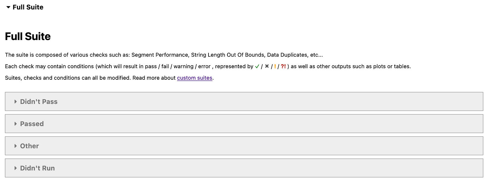
We will explore only parts of the reports, primarily in the Didn’t pass category. We look at the results in the order we presented the resampling techniques.

1. Random undersampling

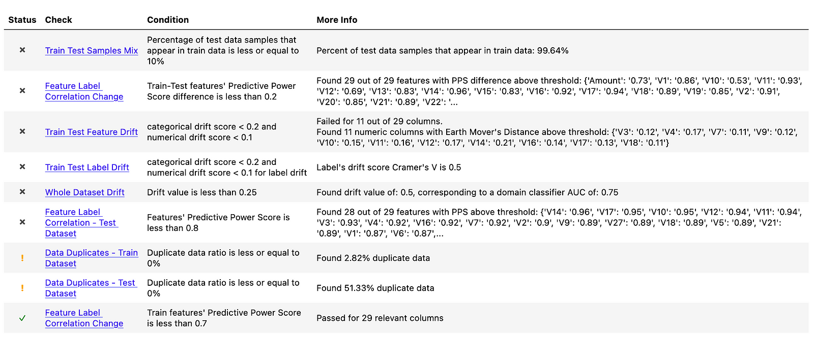
In the table below, we see that quite a few checks failed.

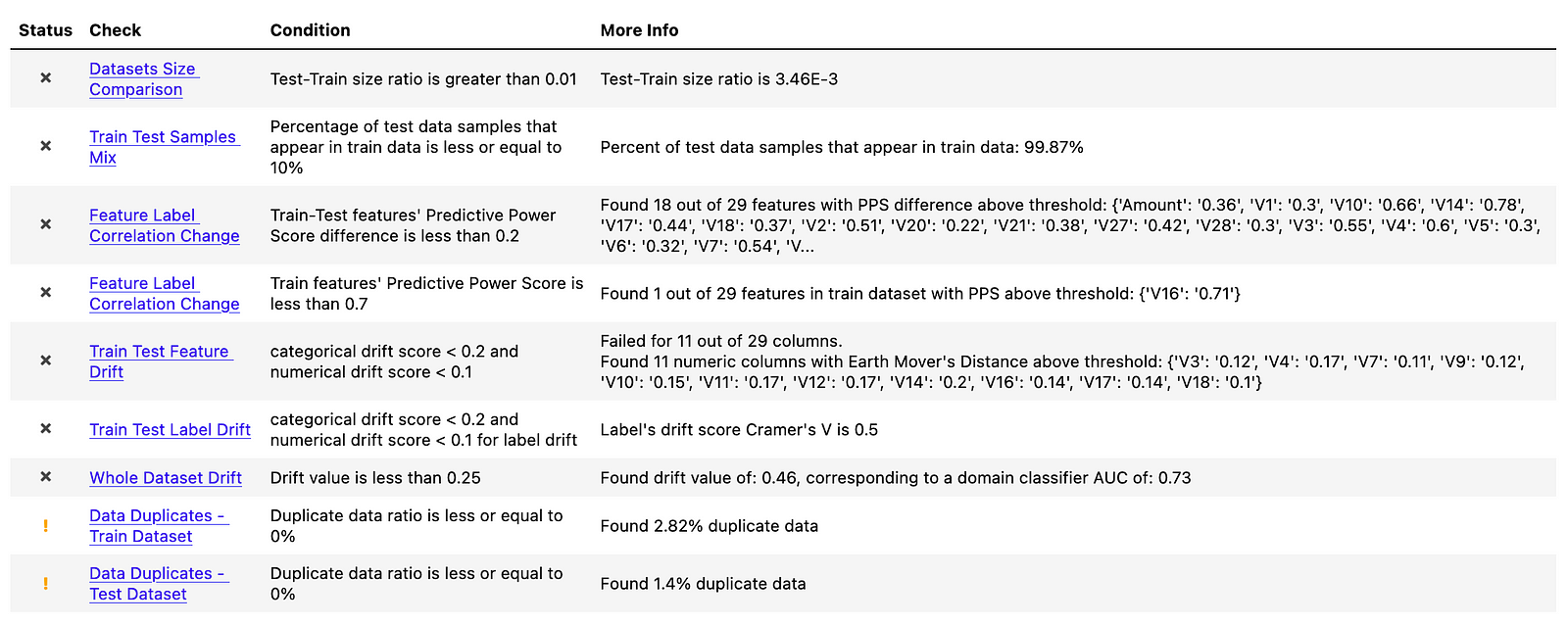
Before diving deeper into some of them, we can address the simpler ones:

• Datasets Size Comparison — this one clearly failed, as the undersampled dataset has 788 observations, while the full one has 227845
• Data Duplicates — Train Dataset and Data Duplicates - Test Dataset — it seems that there are duplicates in the dataset. We should have identified the issue during EDA, but there are indeed duplicated observations in the dataset. However, this has nothing to do with resampling and they were there from the very beginning. In the report, we can see which rows (identified by their indices) are duplicated.
• Train Test Samples Mix — this check investigates if observations in the test data also appear in training data. As the “test” dataset is a resampled one, there is obviously a full overlap of the observations.
• Train Test Label Drift — this check verifies that the distribution of the classes is similar in both datasets. To do so, it uses Cramer’s V. This check naturally failed, as in the original dataset, the positive class is only observed in 0.173% of the observations, while in the resampled dataset the ratio is 50–50.

For our purposes, the most interesting checks are the ones concerning feature/data drift. As we have mentioned, the biggest disadvantage of resampling techniques is that they distort the distribution of the features in the datasets. Furthermore, resampling can not only obscure/alter the relationships between the features themselves, but also the relationship with the target. We can (to some extent) observe that in the following tests.

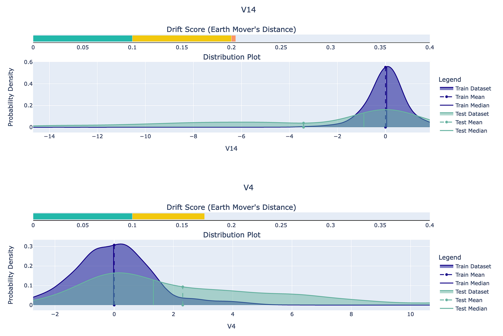
In the Train Test Feature Drift test, we can observe how the distribution of the numerical features differs between the two datasets. The accompanying drift score is simply a measure of the difference between the two distributions. In the following figure, we can see the two features that differ the most between the original and resamples datasets. It is difficult to provide any further interpretation of the differences, as the features were anonymized with the PCA.

To evaluate whether feature drift is present, deepchecks uses the earth mover’s distance (Wasserstein metric) for numerical features and Cramer’s V for categorical features. We will not go into the details of the metrics, as it can be a topic of a separate article. It is also worth mentioning that the feature drift is calculated using a sample of 100000 observations. We can change that value by passing the n_samples argument.

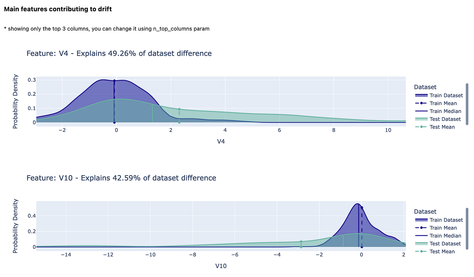
The second test is called Whole Dataset Drift and in it, a separate classifier is trained to distinguish between the two datasets. The features presented in the following figure are the ones that are most important for the domain classifier. The corresponding percentages of the explained dataset difference are the feature importance values calculated using permutation importance. You can read more about permutation importance here.

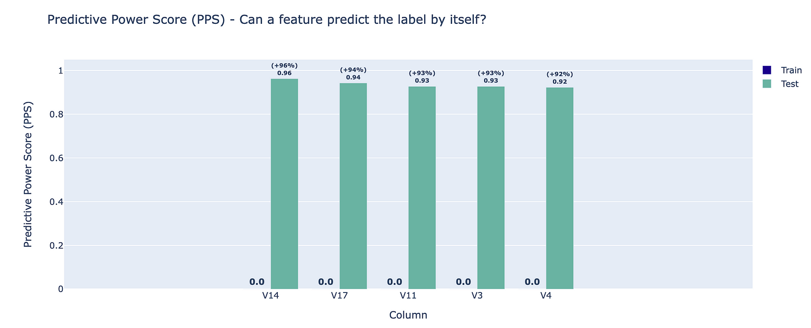
The last interesting test is the Feature Label Correlation Change, which uses the Predictive Power Score to estimate each feature’s ability to predict the target label.

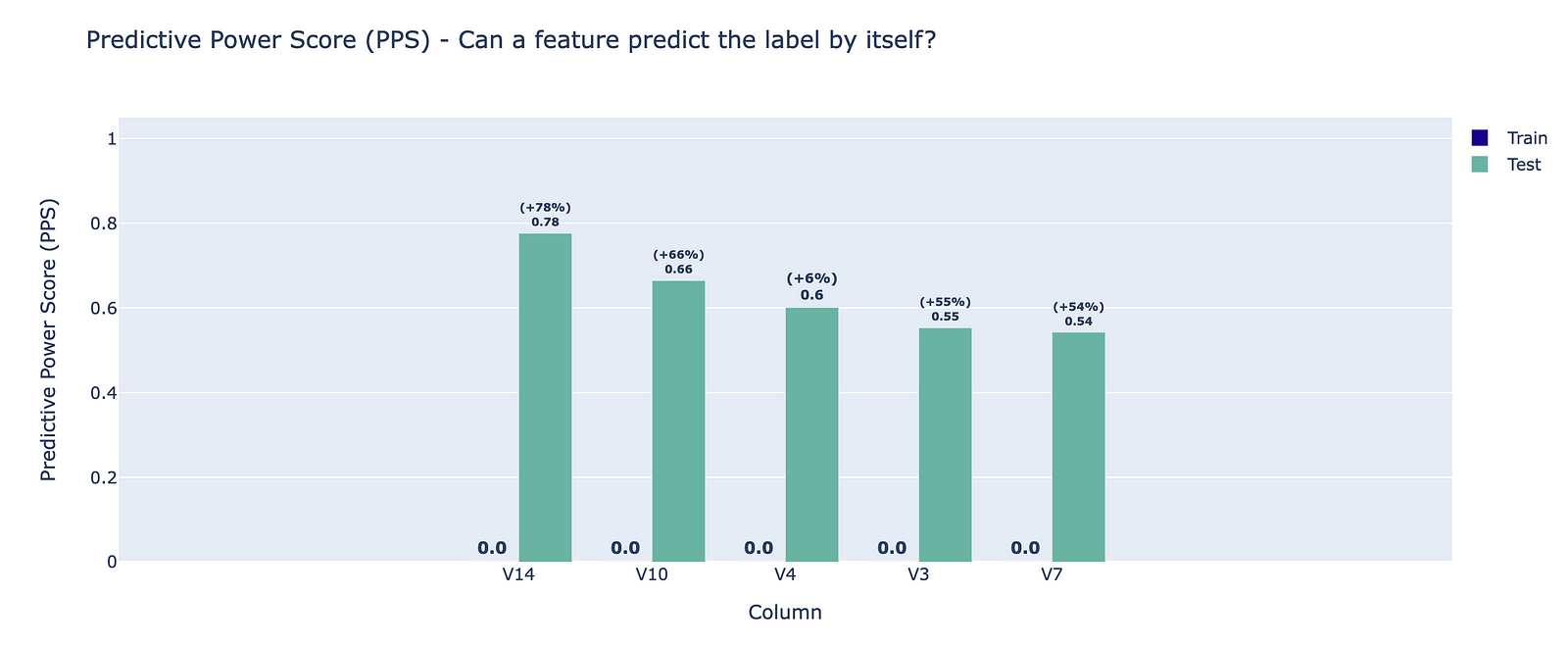
Using the graph and the test summaries (also presented at the beginning of this section), we can draw the following conclusions:

• the PPS for some of the features in the training set is above the determined threshold — normally this is an indication of data leakage, as such a feature might hold information that is based on the target label.
• a large difference between the PPS for two datasets — in the traditional train-test split context, a significantly larger training PPS can be an indication of data leakage. In particular, a larger test PPS can indicate drift in the test set that causes a coincidental correlation with the target.

In the figure, we can see for which 5 features the difference between the original and resampled PPS is the largest. This can be a clear indication of the disadvantage we have mentioned before — creating fake relationships between the features and the target.

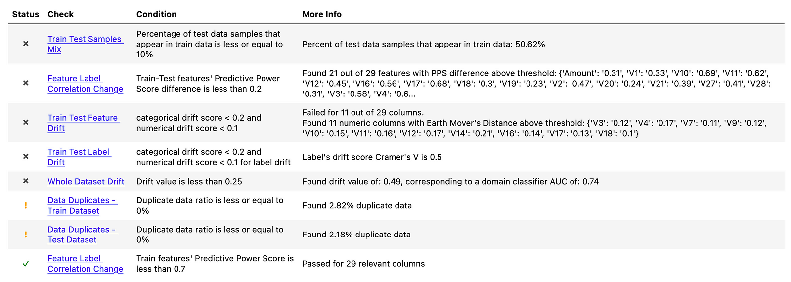
2. Random oversampling

The oversampled dataset suffers from almost the  same set of issues. You can see the summary in the following figure.

Because the issues are very similar, we will only analyze the selected tests. The first one we look into is again the Feature Label Correlation Change. Compared to the random undersampling, this time all features are violating the “Train-Test features’ Predictive Power Score difference is less than 0.2” criterion. As we can see, the PPS values are more extreme for the oversampled dataset. Interestingly, both V14 and V3 features are in the top 5 impacted features for both resampling approaches.

The oversampled dataset is failing a new test, which is also related to the PPS. The Feature Label Correlation — Test Dataset test returns the PPS of all the features in relation to the target. As such, it can be used as an indication of data leakage. For this resampled dataset, 28 out of 29 features are impacted.

3. SMOTE

The dataset resampled with SMOTE also suffers from the majority of the already covered issues. Hence, we will not spend more time covering their meaning.

We will, however, mention the following differences:

• the dataset resampled with SMOTE suffers from the least issues identified by deepchecks.
• the Train Test Samples Mix test has a significantly different value than in the previous cases. Before, we were dealing with almost 100% overlap of the datasets, as we were either duplicating observations or randomly picking some observations from the already available ones. With SMOTE, the value is close to 50%, which intuitively makes sense as approximately half of the observations should be the new, synthetic observations generated by the algorithm.

Automating data validation with GitHub Actions

Running the data validation checks manually every time we change the data can be a bit tedious and error-prone. Thanks to GitHub Actions, we can easily automate that and many other parts of our workflow. For example, we can create an action that runs every time we modify the CSV files (original or resampled) or the data or the scripts used for generating them. Once triggered, the action loads the data versioned with DVC, runs the data validation script, commits the new data validation reports and pushes the changes to the repository. All done automatically with a short YAML script.

You can find the code I used for creating such an action here. In my other article, I have provided a detailed description of the process.

Evaluating the performance of a Random Forest model with various resampling techniques

To make the analysis complete, we also trained a Random Forest model (with the default settings) using the original data and its resampled counterparts. Below we present the evaluation results.

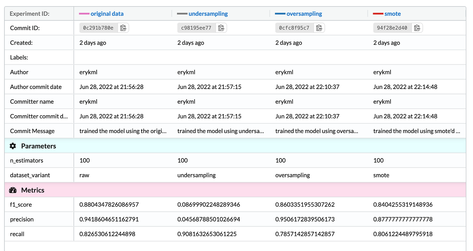
As we are dealing with imbalanced classes, we focused on looking at metrics such as precision, recall, and the F1-Score (the harmonic mean of the former two metrics). After analyzing the results we can state that:

• Not using any resampling approaches resulted in the highest F1-Score on the test set.
• Undersampling resulted in the highest recall, at the cost of very poor precision.
• When it comes to the oversampling approaches, random oversampling resulted in higher precision and the F1-Score than using SMOTE. On the other hand, the synthetic observations from the minority class helped to improve the recall, at a cost of slightly worse precision.

Takeaways

In this article, we presented one of the possible approaches to investigating how various resampling techniques impact the pattern existing in data. As we have seen, resampling can lead to improved model performance when dealing with highly imbalanced classes. However, such approaches also come with a few issues of which we should definitely be aware.

For our analysis, we have used the default checks available in the deepchecks library. The library also offers the possibility of adding custom checks and modifying the thresholds used for identifying issues. This can definitely come in handy when we want to create tailor-made data validation pipelines suiting our needs.

As always, any constructive feedback is more than welcome. You can reach out to me on Twitter. You can find all the code used for this article in this repository.

References

• https://www.kaggle.com/datasets/mlg-ulb/creditcardfraud
• https://docs.deepchecks.com/stable/checks_gallery/tabular.html
• Chawla, N. V., Bowyer, K. W., Hall, L. O., and Kegelmeyer, W. P. (2002). SMOTE: synthetic minority oversampling technique. Journal of artificial intelligence research, 16: 321–357.
• Header Image: Photo by Colton Sturgeon on Unsplash